Despiking Data

Spikes in data can be caused by environmental debris in the water column (phytoplankton, jelly fish, etc.). Regions of high biological productivity are more likely to result in lots of spikes in your data set. Such spikes can change the spectra and skew estimates of dissipation. Despiking detects anomalous, stand alone spikes in data and replaces the spikes and adjoining data points with a carefully constructed average.

The despike function in the ODAS Matlab Library performs the following steps:

  1. The local standard deviation is calculated by a high-pass filtering the input signal, rectifying it, and smoothing it with a low-pass zero-phase filter.
  2. The despike function identifies spikes in the time-domain by comparing the instantaneous rectified signal against a local standard deviation; if the instantaneous signal is above a certain threshold, it is identified as a spike.
  3. The spike and adjoining points are replace by a carefully constructed average.

Steps (1) – (3) are repeated, using the signal produced in step (3) as the input signal for the subsequent iteration of step (1) until no further spikes are identified. This process can be visualized using the ‘-debug’ option of the despike function.

Call the despike function using the command

>> despike(dv, thresh, smooth, Fs, N, ‘-debug’)

where dv is the signal to be despiked, thresh is the threshold value for identifying spikes (quick_look uses a default of 8), smooth is the cut-off frequency of the first order Butterworth filter that is used to smooth the rectified input signal (quick_look uses a default of 50 Hz), Fs is the sampling rate (our instruments usually sample at 512 Hz), and N is the number of spikes removed (quick_look uses a default of N = 0.04*Fs). The spike and adjoining points are replaced by a carefully constructed average. The number of replaced adjoining points is a controllable parameter. If an insufficient number of data points are replaced, spike artifacts will remain in the data and continue to skew the dissipation estimates. If too much data is replaced, the signal variance will be reduced. Effective despiking requires scientific judgement and careful control of despiking parameters to achieve the ideal balance. Appropriately despiked data produces cleaner spectra and more accurate dissipation estimates.

despike_debug copy

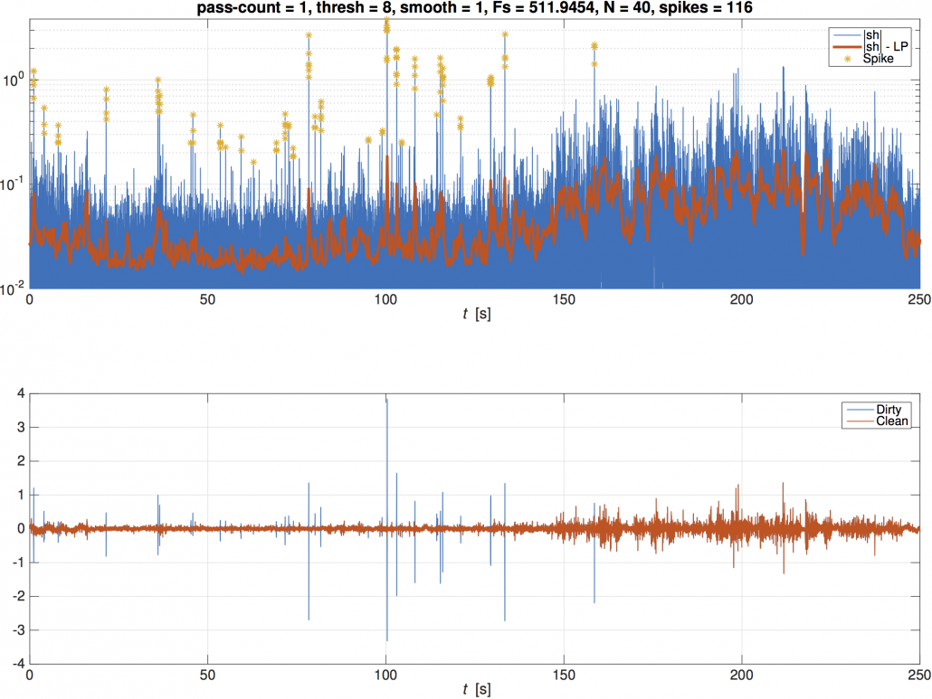
The ‘-debug’ option produces a figure with 2 plots to visualize the despiking processing. The smoothed, rectified data (red) and the instantaneous rectified data (blue) from the first pass of the despiking routine are plotted with identified spikes indicated with a yellow star (top plot). The input signal (blue) and the despiked signal (red) are also plotted (bottom plot). Press any key to move the despiking routine forward to the next pass of the despiking routine. The plots will update to include the despiked signal from the previous iteration being used as the smoothed, rectified signal for the current iteration. The input signal in the lower plot will remain the original input signal.

Use the ‘-debug’ option to test different thresh, smooth, and N parameters. Once you are satisfied with the despiking, the parameters can be input into quick_look to perform the despiking for you.

Converting Raw Data Into Physical Units: odas_p2mat

A second cornerstone of our ODAS Matlab Library 4.0 is the new function odas_p2mat.  odas_p2mat uses the configuration information embedded in the Rockland data file to convert the binary data into data vectors in physical units for both raw signals and derived signals. The data vectors created by odas_p2mat are saved in a mat-file with the same name as the p-file. There are two options for calling odas_p2mat. First, you can call odas_p2mat directly. The mat-file can be analyzed independently, or processed further using quick_look.m. Secondly, you can call quick_look.m, which will then call odas_p2mat.

Upon being called, odas_p2mat first checks if a mat-file already exists with the same name and configuration information as the p-file (see figure blow). If a mat-file exists with matching configuration information that mat-file, the function ends.  If a mat-file exists with different configuration information, odas_p2mat will prompt the user >> Delete MAT file and continue? [y,n] allowing the user to either use the existing mat-file without incorporating the new configuration file, or delete the existing mat-file and use the new configuration information for conversion to physical units. Finally, if a mat-file does not exist, odas_p2mat will create one using the configuration information embedded in the p-file.

odas_p2mat

Note that the processing uses the embedded configuration file string and the calibration parameters contained therein, so these values must be correct.

To call odas_p2mat.m, run the command:

>>odas_p2mat(fname, convert_info);

where ‘fname’ is the name of the file to be processed, and convert_info is the input structure that defines variable processing parameters.

If the convert_info structure is not present when the function is called, default parameters will be used.  The default parameters are appropriate for a vertically profiling VMP; however, they are not appropriate for the MicroRider.  A number of parameters must be adjusted for the MicroRider.

You can create a copy of the default input structure by calling:

>> convert_info = odas_p2mat;

The input structure contains unique parameters that must be adjusted for your particular application.  Please see the ODAS Matlab Library 4.0 Technical Manual for details.

Next week: The new despike.m function, and what does it mean?


A Quick Guide to quick_look.m

A cornerstone of our ODAS Matlab Library 4.0 is the new and improved quick_look.m.  quick_look.m visualizes the content of an RSI data file, the p-file, computes spectra for a selected range, and returns a profile of the rate of dissipation of turbulent kinetic energy.  First, data is converted into physical units by calling the new function odas_p2mat.m.  After data has been converted into physical units, the data from a specified profile (a p-file can contain several profiles) are plotted in several figures to visualize the kinematic properties of profiles, CT data, and microstructure data.  The spectra are plotted against frequency and wavenumber for a defined pressure range.  Finally, the profile of dissipation of kinetic energy is calculated from the shear probes and the results are returned to the user as a large data structure.

quick_look

Please download quick_look.m, along with the rest of our ODAS Matlab Library 4.0, from the Downloads section of our website and try it out to discover new features.  Some new features include:
  • Calls to the new function odas_p2mat.m to convert raw data into physical units;
  • Using the vehicle parameter for choosing application-dependent algorithms;
  • More effective despike routine with new syntax;
  • New profile-defining nomenclature.

Currently quick_look.m handles vertical profiles collected with VMPs, XMPs, and gliders equipped with a MicroRider.  quick_look.m does not handle horizontally profiling instruments, such as a moored profiler (Nemo) or an AUV (Remus). You are also encouraged to peruse the quick_look.m documentation to ensure compatibility with any personal scripts you may have developed.

To call quick_look.m, run the command:

>>diss = quick_look( ‘fname’, P_start, P_end, ql_info);

where diss is the output structure containing the processed data, ‘fname’ is the name of the file to be processing, P_start is the start pressure of the data section used for spectral estimates, P_end is the end pressure of the data section used for spectra estimates, and ql_info is the input structure that defines variable processing parameters.

You can create a copy of the default input structure by calling:

>> ql_info = quick_look;

The input structure contains unique parameters that apply to either quick_look or odas_p2mat, and should be adjusted for your particular application.  Please see the ODAS Matlab Library 4.0 Technical Manual for details.

Next week: Converting raw data into physical units using odas_p2mat

Cheers,
The Customer Success Team

Introducing ODAS Matlab Library 4.0

Welcome! We are very excited to unveil our new website. Please take the time to click around to see what information is new and updated.

This first blog post is an opportunity to introduce you to our exciting new product available on our website: ODAS Matlab Library 4.0. The new ODAS Matlab Library adds a new section to the configuration file, release new matlab functions, and update existing functions. A copy of the new ODAS Matlab Library 4.0 and associated Technical Manual can be downloaded from the Downloads section of our website.

In order to use this new library, you will need to change your instrument configuration file  to include a critical new section and parameter. The new section is called [instrument_info] and only has one required parameter: vehicle. This vehicle parameter is required for converting your raw, binary data into physical units using ODAS Matlab Library 4.0. This section should also be used to provide additional information, such as instrument model, serial number, etc.

vehicle_info_1

The parameter, vehicle, has significant implications in the conversion of data into physical units because the method of estimating the speed of profiling, and data visualization are vehicle dependent. The recognized values for vehicle are vmp, rvmp, slocum_glider, sea_glider, auv, stand, xmp, and nemo. You can familiarize yourself with the new file in the ODAS Matlab Library called default_vehicle_attributes.ini, which describes the default values for each vehicle type. To update the configuration file string in existing p-files, please use the extract_setupstr and patch_setupstr functions.

We have also made significant updates to the existing functions quick_look.m and despike.m. There are two new major functions:

  • odas_p2mat.m, a new function to convert raw data into physical units;
  • show_spec.m, a function that allows you to iterate through the spectra used to calculate the dissipation of turbulent kinetic energy.

Please note that accounts on our old website have NOT been transferred over. You will need to apply (and be approved) for a new account. Once you have access to our Downloads section, you can download the new ODAS Matlab Library 4.0 and Technical Manual.

Next week: What you need to know to use the new quick_look.m.


CF2 Firmware Update

Rockland continually tries to improve its products and services and is pleased to announce an important CF2 firmware update.The new firmware fixes a potential boot failure when using non Silicon Systems brand CompactFlash cards.

Please contact technical support to request the firmware update.

After using your registered user credentials, please proceed to the section titled ‘ODAS5-IR Internal Data Acquisition Software for MR/VMP Instruments’.

Locate the new firmware with the title ‘CF2 Firmware Update (26 March 2010)’ and select ‘Download’.

The resulting ZIP file archive will contain one CF2 application file and one PDF with instructions on how to install the new firmware.