Installing Probes on Rockland Instruments

Installing probes is a critical part of preparing your Rockland instrument for deployment. To help ensure you are using the correct probe installation techniques, we have released instructional videos for our three most common probe holders. Please see details and videos below!

How to Install Probes on the VMP-250: This video covers probe installation on the VMP-250, but it is analogous with probe installation on the VMP-200.


How to Install Probes on the MicroRider-1000: This video covers probe installation on the MicroRider-1000. These probe holder types are also found on the VMP-6000, VMP-500, VMP-2000.


How to Install Probes on the MicroCTD: This video covers probe installation using the Rockland compression plate probe holder design. Although the MicroCTD is used as an example in the video, it is analogous to the MicroRider-1000-G and some custom instruments.


Please Note:

1. The videos do not cover installing probes on the DataHub / MicroPod system. For more instruction to install probes on the MicroPod system please contact Rockland support.

2. Some custom instruments may have specific instructions for probe installation. If you are in doubt, review the manual AND contact Rockland support.

Setup.cfg: Managing Instrument Configuration Files

The instrument configuration file (setup.cfg) is a critical part of your Rockland instrumentation.  Proper management of the configuration file will ensure successful data acquisition. Here are a few tips and tricks for managing configuration files to make your life easier and help ensure successful data collection.


Anatomy of a configuration file:

The first section of a configuration file is known as the root section. The root section determines data acquisition; any changes to this section could create problems with future data collection. We do not advise making changes to the root section, but if you do, please ensure that you test data acquisition on you instrument before deployment. Once you collect data, review it with the ODAS MATLAB Library to confirm successful data acquisition of all channels. Confirming data acquisition is especially important before a glider mission as it may not be possible to modify the setup.cfg file once the glider is at sea. Whenever possible, conduct a short test mission or simulated mission with a modified setup.cfg file before deploying a glider.  We also encourage you to send modified setup.cfg files to the Rockland Support Team for review.

The second section of the configuration file is known as the channel section. It is not critical to have the correct information in this section during data acquisition. The channel section contains all of the coefficients and details required to convert the raw data to physical units during data processing. The contents of this section can be changed after the data has been collected. For example, if you return your shear probes for re-calibration after a deployment, you can insert the new shear probe sensitivity values and re-process the data.


Modifying Configuration Files:


If you need to modify the configuration file in an existing data file (.p files) you can use the extract_setupstr.m function in the ODAS MATLAB Library to extract the configuration file (setup.cfg). The configuration file can then be edited in an a text editor. Notepad++ is a recommended text editor for Windows operating system. Patch the edited configuration file back in to the .p data file using the patch_setupstr.m function.

Whenever modifying the setup.cfg file it is important to record the change as a comment in the header. Comments can also be made anywhere in the configuration file using the semicolon. For Example:

;2019-09-06 Changed S1 sens value, Rockland Support Team

or

; -----------------
; The shear probe channels
[channel]
; instrument dependent parameters
id = 8 
name = sh1
type = shear
adc_fs = 4.096
adc_bits = 16
diff_gain = 0.962
; sensor dependent parameters
sens = 0.0700 ;Comments like this can also be added as needed
SN = M2000
cal_date =2010-01-01

Naming setup.cfg Files and Loading onto the Instrument:


Configuration files can have any name ending with .cfg when they are on your personal computer, however the default name ‘setup.cfg’ must be used when loaded onto the instrument. Rockland has added a new feature to the RSILink software version 4.0.0 to help maintain a configuration file naming convention on your computer. The feature will convert any .cfg file to setup.cfg when it is loaded onto your internally recording instrument. For example: setup_2019_09_06.cfg will be converted to setup.cfg when loaded onto the instrument using RSILink 4.0.0.
Once a modified configuration file has be loaded onto the instrument it is recommended to use the command type setup.cfg in Motocross Terminal to display the contents of the configuration file and check that the modified file has been successfully loaded.
Please contact the Rockland Support team if you have any questions about instrument configuration files or to request a copy of the new version of RSILink.
Sincerely,
Rockland Support Team

How to Zero the Pressure Sensor

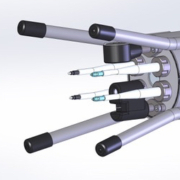
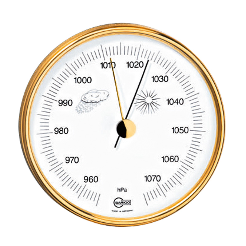
Many oceanographic instruments including those designed by Rockland Scientific, contain pressure sensors. Within Rockland instruments, changes in pressure are sensed as changes in voltage which is converted to units of decibars (dBar) in post processing. The dBar unit is extremely convenient because it is nearly synonymous with water depth in meters (m). At sea level, the Earth’s atmosphere exerts approximately 1 atm (10.1325 dBar) of pressure on the pressure sensor.  However, the Earth’s atmosphere is never at exactly 1 atm because weather systems induce changes in pressure. Low pressure in the atmosphere brings warmth and rain while high pressure brings cool temperatures and clear skies. The range of measured atmospheric pressure at sea level is 10.84 dBar to 8.70 dBar. The pressure sensors in Rockland instrumentation will record these changes in atmospheric pressure and can be used as a barometer!

Due to constant changes in atmospheric pressure the pressure sensors must be zeroed to sea level to accurately measure the water pressure (i. e. depth). When your instrument is first tested at the Rockland production facility the pressure sensor is zeroed to local conditions. However those local conditions may not be consistent with the pressure at the time and location of your measurements. The “zero-ing” of a pressure sensor can be achieved by adjusting one coefficient in your setup.cfg file. This can be accomplished either in post processing or immediately before a deployment (see below). note: The pressure sensor is sensitive to large changes in altitude of the order of 100-1000m , but small changes are insignificant. Thus, you can zero the pressure on the deck of the ship at your deployment site.  

Example: 

The pressure sensor at the time of manufacture is calibrated at near sea level in Victoria, Canada on a rainy day when the atmospheric pressure is 998 mBar; a coef0 value of -3.03 produces a pressure value of zero in these local conditions.  The instrument is shipped to Medellin, Colombia (1495 m above sea level). A deployment in an alpine lake is scheduled for a sunny day when the atmospheric pressure is 1018 mBar. The pressure sensor will need to be zeroed to local conditions by adjusting the coef0 value by 0.2 (dBar). The coef0 is changed to -3.23. The instrument is tested and the pressure now reads zero at the surface.

A few days later a low pressure system moves in but the researchers decide to brave the rain and go out to collect data.  A team member notices that the atmospheric pressure has dropped to 1006 mBar. Now the coef0 must be changed to -3.11 for the pressure value to read zero on the surface of the water.
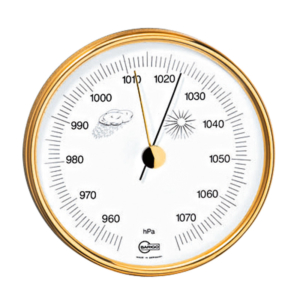
Barometer


Before Deployment

Step 1. Determine the pressure difference from zero: Connect to the instrument via Motocross and start Data Acquisition. The output on the screen will be The Last Record, Next Record and Pressure. Note this pressure value. For real time instruments note the pressure displayed in ODAS4-RT software.

Step 2. Download the Setup.cfg file from the instrument.

Step 3. Add or subtract the pressure difference from Coef0 in the pressure channel 10 in your setup.cfg file. Below is an excerpt from a setup.cfg file. Note that you do not need to change anything in Channel 11.

; —————–

; The pressure transducer

; without pre-emphasis

[channel]

; instrument dependent parameters

id          = 10

name        = P

type        = poly

; sensor dependent parameters

coef0       = -3.03

coef1       = 0.01688

coef2       = 3.888e-8

cal_date    = 2018-12-21

units       = [dBar]

Step 4. Load your new setup.cfg file onto the VMP.

Step 5. Start Data acquisition to check that you have correctly zeroed the pressured.

Post Processing

Step 1. Plot the pressure record in MatLab. We recommend using show_ch(‘filename’, {‘P’}) 

Step 2. On the graph, measure the difference in the pressure record from the time the VMP was on the deck (or in the air) to the 0 dBar line on the graph. If you are using a real time instrument and data acquisition was started in the water, this may not be possible. 

Step 3. Use extract_setupstr(‘filename’, ‘nameofsetupfile’) to extract the setup.cfg file from the .p file. 

Step 3. Add or subtract the pressure difference from Coef0 in the pressure channel 10 in your setup.cfg file. Below is an excerpt from a setup.cfg file. Note that you do not need to change anything in Channel 11.


; —————–

; The pressure transducer

; without pre-emphasis

[channel]

; instrument dependent parameters

id          = 10

name        = P

type        = poly

; sensor dependent parameters

coef0       = -3.03

coef1       = 0.01688

coef2       = 3.888e-8

cal_date    = 1986-05-27

units       = [dBar]


Step 4. Use patch_setupstr(‘filename’, ‘nameofsetupfile’) to patch the new setup.cfg file back into the .p file. 

Step 5. Plot pressure again to check your work.

Remember that pressure sensors are designed for various depth ranges in the ocean. Surpassing the rated depth of a pressure sensor may cause damage to the pressure sensor. For more information contact Rockland Support.

VMP Pressure Sensor Accuracy

The profiling velocity, W, of a VMP instrument is derived using the signal dP/dt from the integrated pressure sensor.  It is imperative to have an accurate and high-resolution sensor to derive the rate of change of pressure, because it is used to convert the shear-probe data into physical units, and to convert the time rate of change of temperature in a vertical gradient of temperature.

Photo Credit: Elanor Frajka-Williams, NOC Southampton

The absolute accuracy of the pressure transducer calibration is 0.1%. The repeatability of the measurements and the polynomial fit to the calibration is accurate 0.01%. However, the pressure transducer has an offset (that is not very temperature dependent) and sensitivity that is temperature dependent. The offset is easily removed by taking a reading in air and adjusting the zeroth-order polynomial coefficient accordingly. The temperature dependence of sensitivity is poorly specified by the manufacturer of the transducer and may be as large as 1% for a temperature change of 20C. This can lead to a possibly significant error in the estimate of the depth, particularly if you are “playing chicken” with the bottom, but the vertical velocity is still accurate to better than 1%.

The estimates of the rate of dissipation of kinetic energy are proportional to the inverse fourth power of the speed of profiling and, therefore, only biased by ~4% by the temperature dependence of sensitivity of the pressure transducer. In comparison, the calibrated sensitivity of the shear probes is accurate to about 5% which leads to a 10% uncertainty in the rate of dissipation. Thus, the pressure transducer provides a satisfactory estimate of the vertical speed of a profiler for the requirements of making dissipation estimates, in an ocean with vertical velocities that are small compared to the fall-rate of a profiler. The last caveat can be important in some situations.

The vertical velocity of the environment is important in highly turbulent flows, such as tidal channels, where horizontal vortices can induce considerable vertical velocity. It is also important in regions of intense internal waves, such as solitons. Consider that in a vertical updraft equal to the fall-rate of a profiler, the rate of change of pressure will be zero. For cases of strong vertical velocity, it may be better to assign a constant speed of profiling equal to the typical fall-rate of a VMP, possibly a rate that is slightly depth dependent to account for the slowing of the profiler from line drag. The hotel-file provides a means of doing so and this is described in Rockland Technical Note TN-039 (available by request).

Finally, the rate of change of pressure, expressed in dbar/s is not exactly equal to the fall-rate of a vertical profiler. The rate of change of pressure with respect to depth is dP/dz = -\⍴ * g. The in situ density, \⍴, varies slightly with depth. The vertical velocity is actually

W = (1e4 /( g \⍴)) dP/dt

when the pressure is expressed in units of dbar. The scaling factor, 1e4/(g \rho) equals [0.9947    0.9883    0.9783    0.9663], for pressures of [ 0 1000 3000 6000] dbar, temperatures of [20 10 0 0] C, and salinity 35. The density effect is inconsequential for depth less than 1000 m and becomes marginally significant at full ocean depth. At full depth, the dissipation estimates are biased low by about 14%. The Rockland library of processing functions does not account for this density effect.

Chlorophyll-a values from CLTU-VMP-250 Nose-Mounted Fluorometer/Optical Backscatter Sensor

The VMP-250 features an integrated compound fluorometer and optical backscatter (OBS) sensor to measure chlorophyll and turbidity.  This CLTU-VMP-250 sensor is co-located on the nose of the profiler with the microstructure sensors and designed for Rockland for vertical profiling applications. 


The CLTU-VMP-250 compound chlorophyll/turbidity sensor uses a light emitting diode for fluorescence and backscattering light.  The CLTU-VMP-250 is factory calibrated with Uranine for Fluoresence and Formazine for Turbidity.  For calibrated characteristics of sensitivity and sensor specifications, see the figure and table below.

Units of Fluorescence:

The short answer is that the unit for the fluorescence intensity is [ppb], i.e. parts per billion, of the uranine concentration. The value in [ppb] is what is reported after running quick_look or convert_odas in the software provided with the VMP-250 instrument.

The extended explanation is that this fluorescence intensity is determined from the raw counts (N) by a linear equation
ppb = A+B*N

where A and B are calibration co-efficients that are in your setup.cfg file. The values of A and B were determined by JFE Advantech Co. Ltd. (the manufacturer of the fluorometer sensor) by comparing the fluorescence signal to a known standard concentration of uranine.  You do not need to worry about implementing this equation because it is already handled by the VMP-250 software.  However, you should verify that the coefficients in your setup file match those in your calibration report.

Converting Fluorescence to Chlorophyll-a:
In order for you to convert to chl-a concentration, you would need to either:

1.  Conduct a literature search to determine how the typical chlorophyl signature of the phytoplankton community at their deployment site relates to concentration of uranine, OR
2.  Collect/filter/analyze for [chl-a] whole water sample at time of deployment and relate to ppb value.

If you have further questions, please email support_at_rocklandscientific.com


Vibrations Sensors: History, Signal Output and Calibration with Rockland Instruments

In 2010, 2-axis piezo-accelerometers (vibration sensors) and a precision inclinometer accurate to 0.1 degrees replaced three DC-response accelerometers in Rockland instruments. The new system produces far better low-frequency angle measurements and a much improved signal-to-noise ratio for higher frequencies. The purpose of the vibration sensors is not to quantify the acceleration of a VMP or MicroRider, but rather to produce a signal that is linear with respect to acceleration so that acceleration-coherent noise can be removed from the environmental signals measured by the shear probe.

The vibration sensors are piezo-ceramic beams that are anchored at one end and have a free cantilevered section over about one-half of their length. We glue a small weight near the tip in order to increase their sensitivity to vibrations. The signals from the beams are treated just like the signal from a shear probe. Thus, the sampled signal is proportional to the rate of change of acceleration and not to acceleration itself.

Rockland does not calibrate the sensors. Their sensitivity can vary by a factor of ~3.

Initially, we used the “type = accel” in the setup.cfg-configuration file to identify the piezo-vibration sensors. However, this is the same type that was used for DC-response accelerometers. This “type” requires two coefficients (coef0 and coef1) to convert the data into physical units. The piezo-accelerometers are not calibrated, so we used coefficients of “coef0=0″ and “coef1=1″, but this is not satisfactory because the second calibration coefficients has units of gravity and, consequently, the raw data are multiplied by a factor of 9.81.

Thus, we added a new signal type, namely “type = piezo”, to the identify the piezo-accelerometers  It does not need any coefficient, but will accept an offset coefficient “coef0 = offset_value”, if available. The main reason for adding this new signal type is to keep the spectra of vibrations on the same scale as the spectra of shear. Many of the plotting functions in the ODAS Matlab Library can detect that the acceleration signals come from piezo-accelerometers and will adjust the scaling of piezo-accelerometer spectra so that they remain visible in a figure of spectra from mixed signals. We thus strongly recommend that you used “type = piezo” in your configuration file. If you use “type = accel” AND use coefficients of 0 and 1, then these functions will assume that the signal comes from a piezo-accelerometer and not from a DC-response accelerometer, for backward compatibility.

The piezo-accelerometrers are inherently AC sensors with a low-frequency cut-off at 0.1 Hz. In addition, we do not know the frequency response of the vibration sensors but estimate that it must be at least to1000 Hz based on the elastic and dimensional properties of the ceramic and the mass that is attached to its tip.

When referring to the the two vibration sensors in a Rockland instrument, we use the nomenclature Ax and Ay because these implied co-ordinates correspond to those of a vertical profiler. If you are using the MicroRider on a glider or an AUV, then the co-ordinates are rotated by 90 degrees around the y-axis. For example, Ax becomes Az, and Ay remains Ay.

Two vibration sensors (Ax and Ay) embedded in front bulkhead block in the nose of the VMP-250 instrument. Signals from Ax and Ay are logged on the ASTP electronics board.

Rockland Customers Tow-Yow-ing the VMP-250

Rockland Scientific instrument users continue to push the operational boundaries of microstructure turbulence measurements.  A sub-section off these microstructure data collection trailblazers have been developing “tow-yow-ing” techniques with the VMP-250 to gather underway profiles in the mixed layer.

1. Oregon State University

Dr. Kipp Shearman, Dr. Johnathan Nash and the Ocean Mixing Group at OSU worked-up a “Tuna Reel” system for tow-yow-ing the VMP-250 to improve the spatial resolution of mixed layer profiles.  This system features the VMP-250 instrument with a Shimano electric fishing reel and a spectra line.  This rig has performed literally thousands of casts and it most recently returned a heavily operated campaign in the Alaska panhandle.

Kipp Shearman operating the OSU Shimano “Tuna Reel” rig for the VMP-250.


2. Tokyo University of Marine Science

In late 2016, Dr. Takeyoshi Nagai tested his idea for an “Underway-VMP”,  using his VMP-250 with the Teledyne Oceanscience Underway CTD winch and standard 1.5mm line.  Preliminary reports show that the system provided good data over two 15-hour tow-yo periods.  Fall speeds of the VMP-250 instrument and single long-brush are approximately 0.76 m/s on average with a “very steady [descent] speed”.  With a slow (i.e. 1-to-2 knots) ship speed, Takeyoshi completed a transect of 300m depth profiles with a 700 – 900m lateral resolution.


Check out more of the exciting research from Prof. Nagai at www.takeyoshi.net


3. University of Minnesota Duluth

Dr. Sam Kelly, who purchased a VMP-250 in early 2017, was intrigued by by OSU’s “Tuna-Reel” rig and the original Peter Gaube “ChUMP” CTD profiling system at the University of Washington Applied Physics Laboratory.  Sam purchased a Lindgren-Pitman S1200 Commercial Electric Reel with a wishbone rod, spectra line and a Optima Blue Top marine battery & charger.  The line is 600 lb braided hollow-core spectra from Lindgren-Pitman, it came pre-spooled.

Basically, there is a chunch of 2,000 lb spectra tied to the instrument and a stainless steel anchor swivel (just outside the tail). The swivel is then attached to the 600 lb line. The 600 lb line is spliced into an end loop (which was tested by UMD and was found to exceed to exceed a 680 lb breaking strength).

The VMP-250 and Lindgren-Pitman rig has been run continuously on 14 day campaigns on Lake Superior.  Each campaign results in roughly 10,000 casts to 50 m.

Two University of Minnesota Duluth students, Taeho Lim (left) and Kaelan Weiss (right), holding the VMP on the back-deck of the R/V Blue Heron in Lake Superior. Dr. Sam Kelly is grabbing a tool in front of them.

A Method for Determining Mixing Rates from Concurrent Temperature & Velocity Measurements

Ocean mixing has historically been estimated using Osborn’s model by measuring the rate of dissipation of turbulent kinetic energy and the background density stratification N while assuming a value of the flux Richardson number, Rif. A constant Rif of 0.17 is typically assumed, despite mounting field, laboratory, and modeling evidence that Rif varies.
This challenge can be overcome by estimating the turbulent diffusivity of heat K_T using the Osborn–Cox model. This model, however, requires measuring the rate of dissipation of thermal variance (chi), which has historically been challenging, particularly in energetic, flows because the high wavenumbers of the temperature gradient spectrum are unresolved due to the limitations of the current technology, i.e. the FP07 sensor:
    • The FP07 temperature signal is attenuated by the sensor and hence getting a true estimate of the signal variance is hard. This attenuation is poorly known and varies from unit to unit (FP07s are made by hand).  Rockland’s quick_look returns the spectrum of the gradient of temperature but this spectrum is not corrected for the response of the FP07 thermistor because there is no consensus on its frequency response.
    • The measured signal depends on the time constant of the FP07 thermistor — the scientific community is still unsure of its value and whether or not the response is single-pole or double-pole.
    • The time constant is speed-dependent because the properties of the boundary layer around the probe (e.g. thickness) are dependent on profiling speed.
    • Integrating the spectrum, without a correction for the response of the FP07, will under estimate the variance of the gradient of temperature and, hence, chi.

Therefore, the probe-dependent attenuation makes it hard to quantity the errors and the uncertainty involved with measuring high-wavenumber temperature gradient spectra.

To overcome this difficulty, a method in the paper Bluteau et al. 2017, Determining Mixing Rates from Concurrent Temperature and Velocity Measurements, is described that determines chi by spectral fitting to the inertial-convective (IC) subrange of the temperature gradient spectra.

While this concept has been exploited for moored time series, particularly near the bottom boundary, it can be used with data collected with gliders, and autonomous and ship-based vertical profilers, from which there are the most measurements.  By using the IC subrange, chi, and hence K_T, can be estimated even in very energetic events.  During less energetic periods, the temperature gradient spectra can also be integrated to obtain chi. In this paper, both of these techniques are used and analyzed for microstructure profiles collected at a site known for its very energetic internal waves. This study demonstrates that the spectral fitting approach resolves intense mixing events with K_T ≥ 10^-2 m2/s.

The validation of this method for microstructure profiling applications will allow Rockland instrument users to utilize their temperature measurements, in conjunction with velocity shear measurements, to calculate mixing rates with reduced error and uncertainty

To overcome this difficulty, a method in the paper Bluteau et al. 2017, Determining Mixing Rates from Concurrent Temperature and Velocity Measurements, is described that determines chi by spectral fitting to the inertial-convective (IC) subrange of the temperature gradient spectra.

While this concept has been exploited for moored time series, particularly near the bottom boundary, it can be used with data collected with gliders, and autonomous and ship-based vertical profilers, from which there are the most measurements.  By using the IC subrange, chi, and hence K_T, can be estimated even in very energetic events.  During less energetic periods, the temperature gradient spectra can also be integrated to obtain chi. In this paper, both of these techniques are used and analyzed for microstructure profiles collected at a site known for its very energetic internal waves. This study demonstrates that the spectral fitting approach resolves intense mixing events with K_T ≥ 10^-2 m2/s.

The validation of this method for microstructure profiling applications will allow Rockland instrument users to utilize their temperature measurements, in conjunction with velocity shear measurements, to calculate mixing rates with reduced error and uncertainty.

The full paper can be found here

UWA Researchers VMP profiling off the coast of Broome, Australia during the Kimberley Internal Soliton Sediment and Mixing Experiment.

Corrosion Prevention: Anodes, Nail-polish, and Continuity Checks

Extreme corrosion on a MicroRider-1000 after a long-term deployment with zinc anodes

Corrosion prevention is an easy to overlook, yet critical practice for operating in the corrosive environment of the ocean. Your Rockland Scientific MicroStructure instrument is equipped with one or more sacrificial anodes to prevent corrosion of your instrument. The anodes are electrically connected to the entire instrument providing protection to the instrument when submerged in seawater.

It is important to note that anode protection only works while the instrument is submerged in seawater.  When the instrument is in air, the anodes stop working and any residual sea water will cause corrosion to occur at vulnerable sites.  For this reason, it is important to thoroughly rinse the instrument with fresh water, especially when it is not active for more than 24 hours.  Before storing the instrument, it is imperative that the instrument is completely dried, as even fresh water (or dampness) can lead to corrosion if left long enough.

Zinc Anode vs. Aluminum Anode

Corrosion study with a MicroRider-1000

In 2015 Rockland Scientific’s Production Tech John Wells conducted an internal study of corrosion affecting Rockland MicroStructure instruments. The key findings of the study are:

  • Aluminum anodes (mil spec. MIL-A-24779) provide superior protection and longevity than zinc anodes
  • Over time zinc anodes build a layer of oxidation that can insulate the anode from seawater diminishing its effectiveness
  • Aluminum anodes are formulated to slough off any oxidation resulting in continued peak performance. 
  • Placing a rubber washer under the anode helps prevent seawater from oxidizing the threads of the anode screw, thereby ensuring a good electrical connection. 

The study findings greatly enhanced the understanding of corrosion prevention at Rockland Scientific. If you have an instrument with an original zinc anode please ensure that the zinc is well scraped off before each deployment. Not all aluminum anodes are created equal, the study determined that a particular anode alloy formulation works best. Rockland recommends that customers source their own spare aluminum anodes with mil spec: MIL-A-24779.  If you would like an aluminum anode to replace a zinc anode on your instrument please contact technical support to request a complimentary aluminum anode and rubber washer.   

Copper tab connecting the rear bulkhead to pressure tube

Consider the anode on the rear bulkhead of a VMP-250. The anode is electrically connected to the rear bulkhead by the threads of its mounting screw. The copper tab on the rear bulkhead contacts the inside of the pressure tube where the anodized layer has been intentionally removed. It is important to check that the copper tab is making a connection to the pressure tube. Overtime the copper tab can become bent and oxidized. The oxidization can easily be removed with sandpaper. You should hear and feel the tab making contact with the tube when the rear bulkhead is inserted into the tube. If you do not hear and feel the tab making contact then gently bend it back into place. You can test if the copper tab is effective by performing the continuity check described below.


Continuity Check

Checking the continuity between the rear bulkhead anode and a scratch on the pressure tube of a MicroRider-1000

Before you deploy your instrument, you can confirm the anode will do it job by performing a continuity check. Use a digital multimeter on the continuity (beep) setting and test for continuity between the anode and any exposed metal such as the rear sealing nut, the front sealing nut, any scratches in the black anodized layer and the connectors on the rear bulkhead. If there is electrical continuity between these parts and the anode then the anode will help protect them from corrosion.   

Nail-polish

It is helpful to have two purposes for everything you bring with you to sea. In addition to making you look your best on deck, nail-polish is effective as a paint to cover nicks and scratches on your instrument. The pressure tube has a black anodized layer that electrically insulates your instrument from seawater. This insulation helps prevent corrosion of your instrument. When the anodized layer is broken, for example from being scratched by sharp fingernails, the exposed metal will start to corrode. To prevent corrosion of exposed metal, thoroughly wash, and dry off, the damaged spot and surrounding area, then paint over with nail-polish. Black nail-polish is often used for aesthetic reasons, but many users prefer a clear polish to allow periodic monitoring of the site.      

Freshwater

Please note that while fresh water is much less corrosive than seawater, proper corrosion prevention practices should still be followed when operating in freshwater bodies. Aluminum anodes will remain effective in freshwater, however for long-term deployments in freshwater Rockland recommends magnesium anodes. Please contact Rockland if you would like to discuss the best option for your application.

Maintenance Tips Review

  • Rinse instrument with freshwater after each deployment
  • Ensure instrument is dry before storing for more than 24hours. Remember, corrosion never sleeps!
  • Perform post cruise maintenance and cleaning before long-term storage
  • Check electrical continuity between anode and sealing nuts and any scratches on pressure tube
  • Bend and sand copper tab on rear bulkhead if necessary
  • Paint any exposed metal due to scratching with nail-polish
  • Scrape oxidization off zinc anodes before each deployment
  • If you have a zinc anode please request a replacement aluminum anode from Rockland
  • Clean the anode bolt and coat threads with anti-seize lubricant such as Never-Seez to ensure continuity between rear bulkhead and anode
  • Magnesium anodes are recommended for long-term freshwater deployments

Troubleshooting Realtime Instruments

Early morning deployment of VMP-2000 using a Chris MacKay hydraulic winch system aboard the R/V Point Sur, Gulf of Mexico 2017

The Rockland suite of instrumentation includes many realtime instruments including the VMP-2000, VMP-500-RT and the VMP-250-RT. Realtime instruments use an electro-mechanical cable to send data back to the ship in real time. Cables can reach lengths up to 2500m and sending data this distance is no easy task. The strength of the received signal on a communication line decreases with increasing length of the line and bit-rate. You can learn more about the transmission of data and modifying the bit-rate in Technical Note 003 available in the downloads section.

The most common issue with realtime instruments are communication errors known as bad buffers. Bad Buffers occur when a data record sent from the instrument is not interpreted correctly by the receiving computer. The data in the record is lost and the cause of the bad buffers must be investigated. Bad buffers are most often caused by damage to the transmission cable. Cables that have been damaged by anomalously large stresses, such as by bending it around sharp-edged objects, or by excessive twisting and hockling, may still show DC electrical characteristics that are nominal. However, the local discontinuity of resistance, capacitance and inductance will cause a partial reflection of the signals. A reflection reduces the amplitude of the transmitted signal. The reflected signal will probably get reflected back into its original direction of travel (by other discontinuities) and thereby skew the phase of the signal received at the far end. This skewing of phase can be very detrimental. Usually, the maximum stress on the cable is at the instrument end. If a cable, that previously worked well, exhibits progressive deterioration (an increase in the frequency of bad buffers, for example), then it may be necessary to trim off some of the cable at the instrument end, and re-terminate in order to re-establish successful communication. The amount trimmed from the cable is usually 50 to 200 m. The entire length of a cable should also be visually inspected for signs of damage, on a regular basis (such as before every cruise), by spooling the cable from the winch to a holding drum.

Directions for re-terminating (splicing) the instrument end of a VMP cable can be found in Technical Note 014 available in the downloads section.